44 how to add data labels to a 3d pie chart in excel
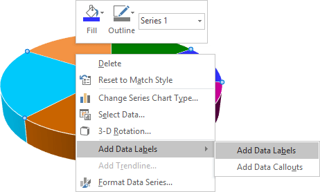
2D & 3D Pie Chart in Excel - Tech Funda To plot the Target data on the chart, select 'Target' series radio button and click 'Apply' button. Similarly, to hide any of the months plots on the chart de-select he checkbox and click on Apply. 3-D Pie Chart To create 3-D Pie chart, select 3-D Pie chart from Insert Chart dropdown (Look at the 1 st picture above). Excel 3-D Pie charts - Microsoft Excel undefined 1. Select the data range (in this example, B3:C8 ). 2. On the Insert tab, in the Charts group, choose the Pie button: Choose the 3-D Pie chart. 3. Right-click in the chart area, then select Add Data Labels and click Add Data Labels in the popup menu: 4. Click in one of the labels to select all of them, then right-click and select Format Data ...
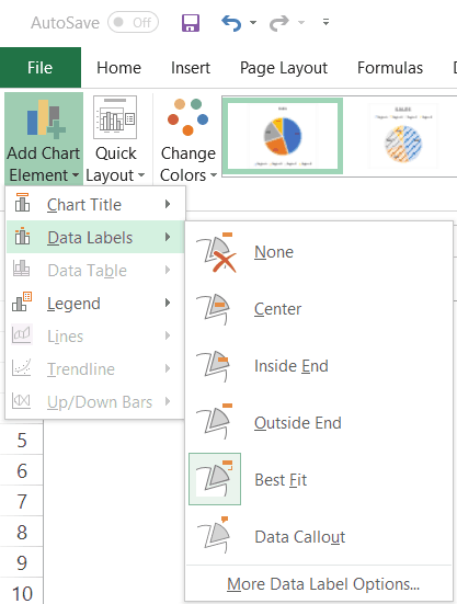
How to Add Data Labels to an Excel 2010 Chart - dummies Use the following steps to add data labels to series in a chart: Click anywhere on the chart that you want to modify. On the Chart Tools Layout tab, click the Data Labels button in the Labels group. None: The default choice; it means you don't want to display data labels. Center to position the data labels in the middle of each data point.

How to add data labels to a 3d pie chart in excel
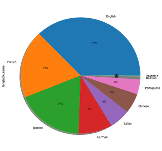
How to show percentage in pie chart in Excel? - ExtendOffice Please do as follows to create a pie chart and show percentage in the pie slices. 1. Select the data you will create a pie chart based on, click Insert > I nsert Pie or Doughnut Chart > Pie. See screenshot: 2. Then a pie chart is created. Right click the pie chart and select Add Data Labels from the context menu. 3. Edit titles or data labels in a chart - support.microsoft.com On a chart, click one time or two times on the data label that you want to link to a corresponding worksheet cell. The first click selects the data labels for the whole data series, and the second click selects the individual data label. Right-click the data label, and then click Format Data Label or Format Data Labels. Pie Chart in Excel | How to Create Pie Chart - EDUCBA Step 1: Select the data to go to Insert, click on PIE, and select 3-D pie chart. Step 2: Now, it instantly creates the 3-D pie chart for you. Step 3: Right-click on the pie and select Add Data Labels. This will add all the values we are showing on the slices of the pie.
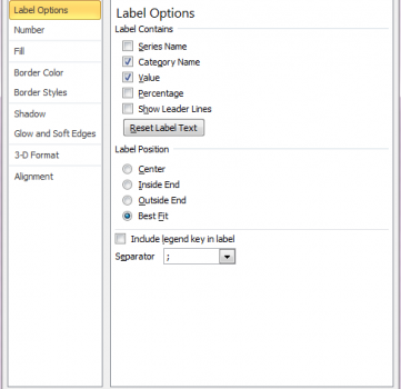
How to add data labels to a 3d pie chart in excel. How to convert the data in Excel table into three-dimensional pie chart ... 1. Open the excel pie chart first and then select the data you want to make. 2. Click Insert - pie chart - 3D pie chart and select the appropriate chart style. 3. Right click the pie chart and click the add data tab to add values. The above is the tutorial of making three-dimensional pie chart with Excel. I hope you like it. Excel charts: add title, customize chart axis, legend and data labels ... To add a label to one data point, click that data point after selecting the series. Click the Chart Elements button, and select the Data Labels option. For example, this is how we can add labels to one of the data series in our Excel chart: For specific chart types, such as pie chart, you can also choose the labels location. How to display leader lines in pie chart in Excel? - ExtendOffice To display leader lines in pie chart, you just need to check an option then drag the labels out. 1. Click at the chart, and right click to select Format Data Labels from context menu. 2. In the popping Format Data Labels dialog/pane, check Show Leader Lines in the Label Options section. See screenshot: 3. Add or remove data labels in a chart - support.microsoft.com Click the data series or chart. To label one data point, after clicking the series, click that data point. In the upper right corner, next to the chart, click Add Chart Element > Data Labels. To change the location, click the arrow, and choose an option. If you want to show your data label inside a text bubble shape, click Data Callout.
How to make a 3D pie chart in Excel - Quora Answer (1 of 4): I have never been a fan of pie charts. Pie charts are intended to show the user group category percentages. Here is an example using Minitab and the tires.mtw data set. This is a pie chart of tire failures by category. In general, users have difficulty comparing percentages due ... How to Rotate Pie Chart in Excel? - WallStreetMojo Move the cursor to the chart area to select the pie chart. Step 5: Click on the Pie chart and select the 3D chart, as shown in the figure, and develop a 3D pie chart. Step 6: In the next step, change the title of the chart and add data labels to it. Step 7: To rotate the pie chart, click on the chart area. How to Create a Pie Chart in Excel - Smartsheet Enter data into Excel with the desired numerical values at the end of the list. Create a Pie of Pie chart. Double-click the primary chart to open the Format Data Series window. Click Options and adjust the value for Second plot contains the last to match the number of categories you want in the "other" category. How to insert data labels to a Pie chart in Excel 2013 - YouTube This video will show you the simple steps to insert Data Labels in a pie chart in Microsoft® Excel 2013. Content in this video is provided on an "as is" basi...
adding decimal places to percentages in pie charts I am V. Arya, Independent Advisor, to work with you on this issue. Right click on your % label - Format Data labels. Beneath Number choose percentage as category. Report abuse. 39 people found this reply helpful. ·. Excel 3-D Pie charts - Microsoft Excel 2016 - OfficeToolTips If you want to create a pie chart that shows your company (in this example - Company A) in the greatest positive light: Do the following: 1. Select the data range (in this example, B5:C10 ). 2. On the Insert tab, in the Charts group, choose the Pie button: Choose 3-D Pie. 3. Right-click in the chart area, then select Add Data Labels and click ... Microsoft Excel Tutorials: Add Data Labels to a Pie Chart To add the numbers from our E column (the viewing figures), left click on the pie chart itself to select it: The chart is selected when you can see all those blue circles surrounding it. Now right click the chart. You should get the following menu: From the menu, select Add Data Labels. New data labels will then appear on your chart: How To Make a Pie Chart in Excel (With Tips) | Indeed.com Select the information and create the chart. Using your mouse, click on the cell in the top left corner and drag until you've highlighted each cell with a category or number in it. Next, click "Insert" at the top left of your window. Depending on the version, you might select "Insert pie or doughnut chart" or an icon of a pie chart, which opens ...
Lesson 2 | How to Create Charts Using Microsoft Excel Tutorial
How to Create and Format a Pie Chart in Excel - Lifewire Jan 23, 2021 · To add data labels to a pie chart: Select the plot area of the pie chart. Right-click the chart. Select Add Data Labels . Select Add Data Labels. In this example, the sales for each cookie is added to the slices of the pie chart. Change Colors

How to make a pie chart in Excel
How to Make a Pie Chart in Excel - WinBuzzer Select your data and press the pie icon in the "Insert" tab of the ribbon. You can then choose which type of pie chart you want. In our case, that's the basic "2-D Pie" option. However ...

How to Make a Pie Chart in Excel: 10 Steps (with Pictures)
How to show data labels in charts created via Openpyxl 2 Answers. This works for me on a line chart (As a combination chart): openpyxls version: 2.3.2: from openpyxl.chart.label import DataLabelList chart2 = LineChart () .... code to build chart like add_data () and: # Style the lines s1 = chart2.series [0] s1.marker.symbol = "diamond" ... your data labels added here: chart2.dataLabels ...

How to Make Pie Charts and Graphs in Excel - BSUPERIOR
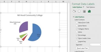
How to Create A 3-D Pie Chart in Excel [FREE TEMPLATE] Right-click on your 3-D pie graph and click " Add Data Labels. " Go to the Label Options tab. Check the " Category Name " box to display the names of the categories along with the actual market share data. Recolor the Slices Next stop: changing the color of the slices.Double-click on the slice you want to recolor and select " Format Data Point. "

3D Pie Chart Excel / Exploded Pie Chart Replacement - Peltier Tech Blog : 3d excel pie chart for ...
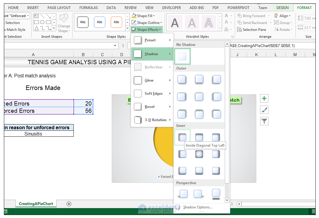
How to Make a Pie Chart in Excel & Add Rich Data Labels to The Chart! Creating and formatting the Pie Chart. 1) Select the data. 2) Go to Insert> Charts> click on the drop-down arrow next to Pie Chart and under 2-D Pie, select the Pie Chart, shown below. 3) Chang the chart title to Breakdown of Errors Made During the Match, by clicking on it and typing the new title.

Pie Chart – Excel Tutorials
Creating Pie Chart and Adding/Formatting Data Labels (Excel) Creating Pie Chart and Adding/Formatting Data Labels (Excel) Creating Pie Chart and Adding/Formatting Data Labels (Excel)

Excel 3-D Pie Charts - Microsoft Excel undefined
Display data point labels outside a pie chart in a paginated report ... Create a pie chart and display the data labels. Open the Properties pane. On the design surface, click on the pie itself to display the Category properties in the Properties pane. Expand the CustomAttributes node. A list of attributes for the pie chart is displayed. Set the PieLabelStyle property to Outside. Set the PieLineColor property to Black.

CD: Pie of Pie Charts
Pie Chart in Excel | How to Create Pie Chart - EDUCBA Step 1: Select the data to go to Insert, click on PIE, and select 3-D pie chart. Step 2: Now, it instantly creates the 3-D pie chart for you. Step 3: Right-click on the pie and select Add Data Labels. This will add all the values we are showing on the slices of the pie.
30 How To Label A Pie Chart - Labels For You
Edit titles or data labels in a chart - support.microsoft.com On a chart, click one time or two times on the data label that you want to link to a corresponding worksheet cell. The first click selects the data labels for the whole data series, and the second click selects the individual data label. Right-click the data label, and then click Format Data Label or Format Data Labels.
How to Make a Pie Chart in Excel & Add Rich Data Labels to The Chart!
How to show percentage in pie chart in Excel? - ExtendOffice Please do as follows to create a pie chart and show percentage in the pie slices. 1. Select the data you will create a pie chart based on, click Insert > I nsert Pie or Doughnut Chart > Pie. See screenshot: 2. Then a pie chart is created. Right click the pie chart and select Add Data Labels from the context menu. 3.
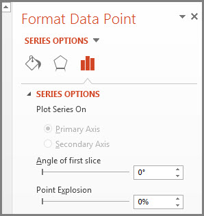
Rotate a pie chart - Office Support

Excel 3-D Pie Charts
4.1 Choosing a Chart Type – Beginning Excel
How to Make a PIE Chart in Excel (Easy Step-by-Step Guide)
Excel 3-D Pie Charts
Excel -3- Figures and graphs – bioST@TS

How to Make Pie Charts and Graphs in Excel - BSUPERIOR
Post a Comment for "44 how to add data labels to a 3d pie chart in excel"