38 accept labels in formulas excel 2013

› mail-merge-labels-from-excelHow to mail merge and print labels from Excel - Ablebits Apr 22, 2022 · When done, click the OK button.; Step 3. Connect to Excel mailing list. Now, it's time to link the Word mail merge document to your Excel address list. On the Mail Merge pane, choose the Use an existing list option under Select recipients, click Browse… and navigate to the Excel worksheet that you've prepared. Excel 2013, Filter not working for all table content Select the "Table tools" ribbon that is displayed above the other ribbons. Select "Resize table" (at far left of Table tools ribbon). The resize dialog will be displayed. It will be obvious it only rows down to 468 are included in the table by the range shown by default as the current range of the table.

stackoverflow.com › questions › 15013911Creating a chart in Excel that ignores #N/A or blank cells Excel 2013 allows you to filter a chart's data without messing with the worksheet. In this case you'll be able to block plotting of the category with the errors. I don't know if you can do it dynamically, since the UI for it has boxes for you to check. No help if you're stuck with 2007/10. –

Accept labels in formulas excel 2013

Excel refuses to accept formula - Microsoft Tech Community Excel refuses to accept formula When I type in a or insert a formula, even if exactly off an Excel tutorial, it shows: "You've entered too few arguments" and I cannot get it to calculate any formula. I am trying to do a simple Countif calculation on a small dataset. I use Office 365 Version 18.2106.12410. and an updated 2021 Excel. Jan's Excel Format & Arrange (97- 2003): Exercises [Hint: Cut and Insert Cells.] There should be a blank row between the Totals and Expenses rows. Move the column labels from below Expenses to above Income. Insert: Between the columns Category and Budget, insert 2 columns. Label the columns Budget Quantity and Budget Cost each and wrap the text. Define and use names in formulas - support.microsoft.com Select Formulas > Create from Selection. In the Create Names from Selection dialog box, designate the location that contains the labels by selecting the Top row,Left column, Bottom row, or Right column check box. Select OK. Excel names the cells based on the labels in the range you designated. Use names in formulas

Accept labels in formulas excel 2013. Enable or Disable Excel Data Labels at the click of a button - How To Select and to go Insert tab > Charts group > Click column charts button > click 2D column chart. This will insert a new chart in the worksheet. Step 2: Having chart selected go to design tab > click add chart element button > hover over data labels > click outside end or whatever you feel fit. This will enable the data labels for the chart. Excel Workbook wouldn't accept cumulated total formula (Eg. - Microsoft ... Excel Workbook wouldn't accept cumulated total formula (Eg. =SUM ('Musoma Municipal:Butiama District'!D15) from its sheets. Hi, I have been using Excel over 20 years now though I can't say that I know Excel that much. I have recently denied by Excel to make formula that I have been using over four years now, work. AutoFill in Excel - How to Use? (Top 5 Methods with Examples) Fill the range A26:A34 with a series of time values incrementing by one hour. Use the "fill series" option of the AutoFill feature in excel. Step 1: Select cell A25. Step 2: Drag the fill handle till cell A34. Excel has filled the range A26:A34 with the different time values, as shown in the succeeding image. How to use cell references and defined names in criteria in Excel ... =$D$1 To use the value of a defined name, such as "CritVar", type the following formula in the criteria cell: =CritVar To use the operators, such as less than (<) and greater than (>), the operator must be concatenated with the formula.

Keep Your Formulas From Shifting In Excel - Business Insider Aug 2, 2013, 12:08 PM One of the best features in Excel is the ability to plug in a formula and then easily drag it into new cells and have it automatically shift to the corresponding cell values.... › blog › 50-things-you-can-do50 Things You Can Do With Excel Pivot Table - MyExcelOnline Jul 18, 2017 · What is a Pivot Table? Pivot Tables in Excel are one of the most powerful features within Microsoft Excel. An Excel Pivot Table allows you to analyze more than 1 million rows of data with just a few mouse clicks, show the results in an easy to read table, “pivot”/change the report layout with the ease of dragging fields around, highlight key information to management and include Charts ... How to use AutoFill in Excel - all fill handle options - Ablebits In Excel 2010-2013 click File -> Options -> Advanced -> scroll to the General section to find the Edit Custom Lists… button. Since you already selected the range with your list, you will see its address in the Import list from cells: field. Press the Import button to see your series in the Custom Lists window. › how-to-group-in-excel-4691532How to Group in Excel - Lifewire Jul 15, 2020 · Instructions in this article apply to Excel 2019, 2016, 2013, 2010, 2007; Excel for Microsoft 365, Excel Online and Excel for Mac. Grouping in Excel You can create groups by either manually selecting the rows and columns to include, or you can get Excel to automatically detect groups of data.

How to Prevent or Disable Auto Fill in Table Formulas - Excel Campus Go to the File tab on the Ribbon. Choose Options. Choose Proofing. Click on the AutoCorrect Options button. Choose the AutoFormat As You Type tab (if not already selected). Check the box that says Fill formulas in tables to create calculated columns. Hit OK. How to Assign a Name to a Range of Cells in Excel To assign a name to a range of cells, select the cells you want to name. The cells don't have to be contiguous. To select non-contiguous cells, use the "Ctrl" key when selecting them. Click the mouse in the "Name Box" above the cell grid. Type a name for the range of cells in the box and press "Enter". Understanding Date-Based Axis Versus Category-Based Axis in Trend ... The fill handle is the square dot in the lower-right corner of the active cell indicator. Excel copies the formula from cell B2 down to your range of dates. Select Column B2. On the Home tab, select the drop-down at the top of the Number group and choose either Short Date or Long Date. Excel displays the numbers in Column B as a date (see ... Use defined names to automatically update a chart range - Office Microsoft Excel 97 through Excel 2003. On the Insert menu, click Chart to start the Chart Wizard. Click a chart type, and then click Next. Click the Series tab. In the Series list, click Sales. In the Category (X) axis labels box, replace the cell reference with the defined name Date. For example, the formula might be similar to the following ...

Excel 2003 Printing Options

excel - Change format of all data labels of a single series at once ... Click anywhere in formula bar above. Don't change anything. Click the 'tick icon' just to the left of the formula bar. Go straight back to the same data series and right mouse click, and choose add data labels This has worked in Excel 2016. Purely by luck I worked this out saving a great deal of time and frustration. Share

Advanced Excel Formulas - DCOUNT Function Description With Example

› data-definition-excel-3123415Excel Spreadsheet Data Types - Lifewire Feb 07, 2020 · Formulas are mathematical equations that work in combination with data from other cells on the spreadsheet. Simple formulas are used to add or subtract numbers. Advanced formulas perform algebraic equations. Spreadsheet functions are formulas that are built into Excel.

Where Do I Put The Label? In Excel – Excel-Bytes

How to Print Labels From Excel - EDUCBA Navigate towards the folder where the excel file is stored in the Select Data Source pop-up window. Select the file in which the labels are stored and click Open. A new pop up box named Confirm Data Source will appear. Click on OK to let the system know that you want to use the data source. Again a pop-up window named Select Table will appear.

Excel Tips and Tricks: 2012

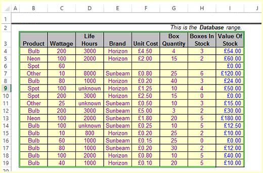
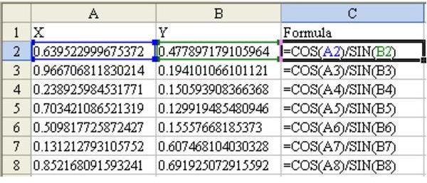
Excel- Labels, Values, and Formulas - WebJunction Simple Formula: Click the cell in which you want the answer (result of the formula) to appear. Press Enter once you have typed the formula. All formulas start with an = sign. Refer to the cell address instead of the value in the cell e.g. =A2+C2 instead of 45+57. That way, if a value changes in a cell, the answer to the formula changes with it.

How to Use Excel Like a Pro: 18 Easy Excel Tips, Tricks, & Shortcuts

Excel named range - how to define and use names in Excel If your data is arranged in a tabular form, you can quickly create names for each column and/or row based on their labels: Select the entire table including the column and row headers. Go to the Formulas tab > Define Names group, and click the Create from Selection button. Or, press the keyboard shortcut Ctrl + Shift + F3.

One of the keys to all happiness, is to have a bad memory...: Excel

IFS Function in Excel 2016, 2013, 2010 and 2007 - Office PowerUps Excel 365 or Excel 2019 introduced a new function called IFS. You can add an IFS function in Excel 2016, 2013 or your copy of Excel 2010, or 2007 with the Excel PowerUps add-in. This IFS function in Excel 2016 (or earlier) allows you to specify a series of conditions easily in a single function without having to nest several IF functions.

Using Labels to Simplify Your Excel 2003 Formulas

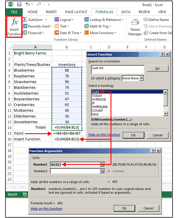
Excel 2016 - How to Use Formulas and Functions To do this, we are going to click Insert Function on the Ribbon under the Formulas tab. Once again, we enter "average of cells" in the "Search for a Function field," then click the Go button. Select Average, then click OK. Excel prompts us for our arguments. The arguments are the cells or values that we want to use to calculate the function.

Discover How To Assign A Formula To A Name With This Excel Tutorial

› blog › 61-excel-charts-examples61 Excel Charts Examples! | MyExcelOnline Aug 28, 2020 · Learn the most popular Excel Formulas ever: VLOOKUP, IF, SUMIF, INDEX/MATCH, COUNT, SUMPRODUCT plus more 101 Ready To Use Excel Macros E-Book Access 101 Ready To Use Macros with VBA code which you can Copy & Paste to your workbooks straight away

Your Excel formulas cheat sheet: 22 tips for calculations and common tasks | PCWorld

Adding rich data labels to charts in Excel 2013 - Microsoft 365 Blog To add a data label in a shape, select the data point of interest, then right-click it to pull up the context menu. Click Add Data Label, then click Add Data Callout . The result is that your data label will appear in a graphical callout. In this case, the category Thr for the particular data label is automatically added to the callout too.

Share :