43 display data labels in excel
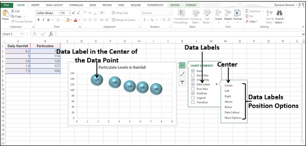
› charts › dynamic-chart-dataCreate Dynamic Chart Data Labels with Slicers - Excel Campus Feb 10, 2016 · Typically a chart will display data labels based on the underlying source data for the chart. In Excel 2013 a new feature called “Value from Cells” was introduced. This feature allows us to specify the a range that we want to use for the labels. Since our data labels will change between a currency ($) and percentage (%) formats, we need a ... Quick Tip: Excel 2013 offers flexible data labels | TechRepublic right-click and choose Insert Data Label Field. In the next dialog, select. [Cell] Choose Cell. When Excel displays the source dialog, click the cell that. contains the MIN () function, and click ...
› documents › excelHow to hide zero data labels in chart in Excel? - ExtendOffice 1. Right click at one of the data labels, and select Format Data Labels from the context menu. See screenshot: 2. In the Format Data Labels dialog, Click Number in left pane, then select Custom from the Category list box, and type #"" into the Format Code text box, and click Add button to add it to Type list box. See screenshot: 3.

Display data labels in excel
Change the format of data labels in a chart To get there, after adding your data labels, select the data label to format, and then click Chart Elements > Data Labels > More Options. To go to the appropriate area, click one of the four icons ( Fill & Line, Effects, Size & Properties ( Layout & Properties in Outlook or Word), or Label Options) shown here. Create Dynamic Chart Data Labels with Slicers - Excel Campus Feb 10, 2016 · Typically a chart will display data labels based on the underlying source data for the chart. In Excel 2013 a new feature called “Value from Cells” was introduced. This feature allows us to specify the a range that we want to use for the labels. Since our data labels will change between a currency ($) and percentage (%) formats, we need a ... Add or remove data labels in a chart - support.microsoft.com Right-click the data series or data label to display more data for, and then click Format Data Labels. Click Label Options and under Label Contains , select the Values From Cells checkbox. When the Data Label Range dialog box appears, go back to the spreadsheet and select the range for which you want the cell values to display as data labels.
Display data labels in excel. › pivot-table-filterPivot Table Filter in Excel | How to Filter Data in a Pivot ... Here, we discuss how to filter data in a PivotTable with the help of examples and a downloadable Excel template. You may learn more about Excel from the following articles: – Excel Pivot Table From Multiple Sheets Excel Pivot Table From Multiple Sheets Pivot Table is a basic data analysis tool that calculates, summarizes, & analyses the data ... Data Labels in Power BI - SPGuides Nov 20, 2019 · Value decimal places: The Value decimal places always should be in Auto mode. Orientation: This option helps in which view you want to see the display units either in Horizontal or in Vertical mode. Position: This option helps to select your position of the data label units. Suppose, you want to view the data units at the inside end or inside the center, then you can … Edit titles or data labels in a chart - support.microsoft.com The first click selects the data labels for the whole data series, and the second click selects the individual data label. Right-click the data label, and then click Format Data Label or Format Data Labels. Click Label Options if it's not selected, and then select the Reset Label Text check box. Top of Page How to hide zero data labels in chart in Excel? - ExtendOffice 1. Right click at one of the data labels, and select Format Data Labels from the context menu. See screenshot: 2. In the Format Data Labels dialog, Click Number in left pane, then select Custom from the Category list box, and type #"" into the Format Code text box, and click Add button to add it to Type list box. See screenshot: 3.
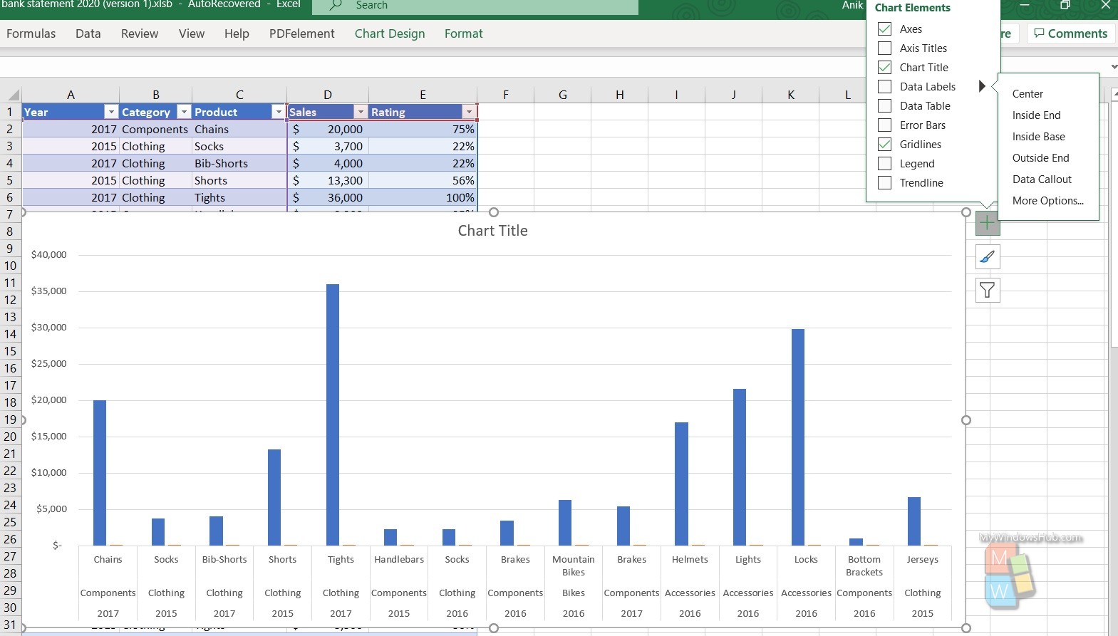
How to add or move data labels in Excel chart? - ExtendOffice 2. Then click the Chart Elements, and check Data Labels, then you can click the arrow to choose an option about the data labels in the sub menu. See screenshot: In Excel 2010 or 2007. 1. click on the chart to show the Layout tab in the Chart Tools group. See screenshot: 2. Then click Data Labels, and select one type of data labels as you need ... How to add data labels from different column in an Excel chart? Right click the data series in the chart, and select Add Data Labels > Add Data Labels from the context menu to add data labels. 2. Click any data label to select all data labels, and then click the specified data label to select it only in the chart. 3. What Are Data Labels in Excel (Uses & Modifications) - ExcelDemy For more data, right-click the series or label you would like to display, and then click on the Format Data Labels. Then, go to the Label Options > Label Contains > Values From Cells. Select the cell values you wish to display as data labels from the Data Label Range window appear. 10 spiffy new ways to show data with Excel | Computerworld Apr 13, 2018 · 10 spiffy new ways to show data with Excel ... Right-click the X-axis labels and click Format Axis. In the Axis Options pane, click the Number item and, in Category, select Date from the drop-down ...
Excel tutorial: How to use data labels Generally, the easiest way to show data labels to use the chart elements menu. When you check the box, you'll see data labels appear in the chart. If you have more than one data series, you can select a series first, then turn on data labels for that series only. You can even select a single bar, and show just one data label. How to Add Data Labels in Excel - Excelchat | Excelchat In Excel 2013 and the later versions we need to do the followings; Click anywhere in the chart area to display the Chart Elements button Figure 5. Chart Elements Button Click the Chart Elements button > Select the Data Labels, then click the Arrow to choose the data labels position. Figure 6. How to Add Data Labels in Excel 2013 Figure 7. Add or remove data labels in a chart - support.microsoft.com Right-click the data series or data label to display more data for, and then click Format Data Labels. Click Label Options and under Label Contains, select the Values From Cells checkbox. When the Data Label Range dialog box appears, go back to the spreadsheet and select the range for which you want the cell values to display as data labels. › article › 326866410 spiffy new ways to show data with Excel | Computerworld Apr 13, 2018 · In-cell charts are like a heads-up display for your data, providing an immediate visual context in spreadsheets. The Sparkline feature, introduced in Excel 2013, lets you select data from rows or ...
31 What Is Data Label In Excel - Labels Database 2020
How to Automatically Update Data in Another Sheet in Excel Linking data in a real data set is more complex and depends on your situation. You might need to use techniques other than those listed above. If you are in a rush and want your problem answered by an Excel expert, try our service. The experts are available to help you 24/7. The first question is free.

How to Create a MS Excel 2010 Pivot Table – An Introduction | Technical Communication Center ...
TOP 9 what are data labels in excel BEST and NEWEST - Kiến Thức Về ... 4.About Data Labels. Author: . Post date: 2 yesterday. Rating: 4 (1925 reviews) Highest rating: 5. Low rated: 1. Summary: Data labels are text elements that describe individual data points. Displaying data labels. You may display data labels for all data points in the chart, for ….
November 2018
Always-on security monitoring and alerts. Extended 1-year version history and file recovery. Plus all the storage space you need. Dropbox Advanced is a secure collaboration solution for your entire team.
How To Show Or Hide Data Labels On MS Excel? | My Windows Hub
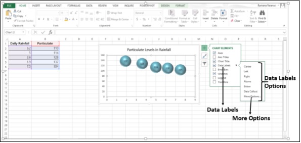
How to Add Data Labels to Scatter Plot in Excel (2 Easy Ways) - ExcelDemy Then, go to the Insert tab. After that, select Insert Scatter (X, Y) or Bubble Chart > Scatter. At this moment, we can see the Scatter Plot visualizing our data table. Secondly, go to the Chart Design tab. Now, select Add Chart Element from the ribbon. From the drop-down list, select Data Labels.

Custom data labels in a chart | Get Digital Help - Microsoft Excel resource
Dropbox.com Work efficiently with teammates and clients, stay in sync on projects, and keep company data safe—all in one place. Get Dropbox for work. For personal use. Keep everything that’s important to you and your family shareable and safe in one place. Back up files in the cloud, share photos and videos, and more. ...

GANTT Procedure
Data Labels in Excel Pivot Chart (Detailed Analysis) 7 Suitable Examples with Data Labels in Excel Pivot Chart Considering All Factors 1. Adding Data Labels in Pivot Chart 2. Set Cell Values as Data Labels 3. Showing Percentages as Data Labels 4. Changing Appearance of Pivot Chart Labels 5. Changing Background of Data Labels 6. Dynamic Pivot Chart Data Labels with Slicers 7.
Excel Dashboards - Краткое руководство - CoderLessons.com
How to change axis labels order in a bar chart - Microsoft Excel 365 See more about the competition chart. To change the order of the labels on the axis, do the following: 1. Right-click the horizontal axis and click the Format Axis... in the popup menu (or double-click the axis): 2. On the Format Axis pane, on the Axis Options tab, in the Axis Options group: Under Axis position, select the Category in reverse ...

Format Number Options for Chart Data Labels in Excel 2011 for Mac
How to add data labels from different column in an Excel chart? This method will introduce a solution to add all data labels from a different column in an Excel chart at the same time. Please do as follows: 1. Right click the data series in the chart, and select Add Data Labels > Add Data Labels from the context menu to add data labels. 2.
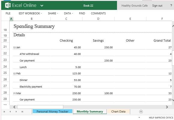
Personal Money Spending Tracker Template For Excel Online
How to Change Excel Chart Data Labels to Custom Values? - Chandoo.org May 05, 2010 · Now, click on any data label. This will select “all” data labels. Now click once again. At this point excel will select only one data label. Go to Formula bar, press = and point to the cell where the data label for that chart data point is defined. Repeat the process for all other data labels, one after another. See the screencast.
Custom data labels in a chart | Get Digital Help - Microsoft Excel resource
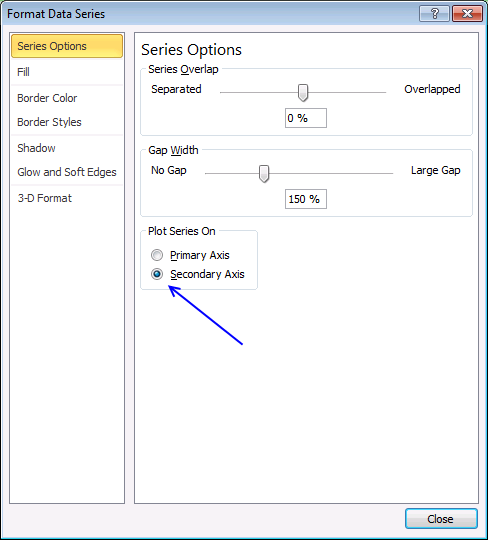
Data labels on small states using Maps - Microsoft Community Data labels on small states using Maps. Hello, I need some assistance using the Filled Maps chart type in Excel (note: this is NOT Power Maps). I have some data (see attachment below) that I've plotted on a map of the USA. Because the data only applied to 7 states I changed the "map area" (under Format Data Series-->Series Options) to show ...

How to Create a Year Over Year Comparison Bar Chart in Excel?
How to add data labels in excel to graph or chart (Step-by-Step) Add data labels to a chart. 1. Select a data series or a graph. After picking the series, click the data point you want to label. 2. Click Add Chart Element Chart Elements button > Data Labels in the upper right corner, close to the chart. 3. Click the arrow and select an option to modify the location. 4.

Pie Chart - PK: An Excel Expert
How to Add Data Labels to an Excel 2010 Chart - dummies On the Chart Tools Layout tab, click Data Labels→More Data Label Options. The Format Data Labels dialog box appears. You can use the options on the Label Options, Number, Fill, Border Color, Border Styles, Shadow, Glow and Soft Edges, 3-D Format, and Alignment tabs to customize the appearance and position of the data labels.

How to Create Progress Charts (Bar and Circle) in Excel - Automate Excel
Add data labels and callouts to charts in Excel 365 - EasyTweaks.com Step #3: Format the data labels. Excel also gives you the option of formatting the data labels to suit your desired look if you don't like the default. To make changes to the data labels, right-click within the chart and select the "Format Labels" option.
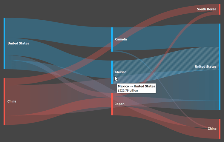
WinForms Sankey Diagram - Data Visualization for .NET | DevExpress
Pivot Table Filter in Excel | How to Filter Data in a Pivot Table ... Here, we discuss how to filter data in a PivotTable with the help of examples and a downloadable Excel template. You may learn more about Excel from the following articles: – Excel Pivot Table From Multiple Sheets Excel Pivot Table From Multiple Sheets Pivot Table is a basic data analysis tool that calculates, summarizes, & analyses the data ...
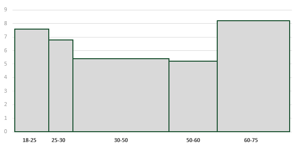
Variable width column charts and histograms in Excel - Excel off the grid
chandoo.org › wp › change-data-labels-in-chartsHow to Change Excel Chart Data Labels to Custom Values? May 05, 2010 · Now, click on any data label. This will select “all” data labels. Now click once again. At this point excel will select only one data label. Go to Formula bar, press = and point to the cell where the data label for that chart data point is defined. Repeat the process for all other data labels, one after another. See the screencast.
Advanced Excel - более богатые метки данных - CoderLessons.com
How to Display Percentage in an Excel Graph (3 Methods) Display Percentage in Graph. Select the Helper columns and click on the plus icon. Then go to the More Options via the right arrow beside the Data Labels. Select Chart on the Format Data Labels dialog box. Uncheck the Value option. Check the Value From Cells option.
Post a Comment for "43 display data labels in excel"